Introduction
Linear inverse problems are ubiquitous in science and engineering, with applications ranging from medical imaging to astronomy and remote sensing. These problems typically involve recovering an unknown signal $\bm{x}^* \in \mathbb{R}^n$ from noisy linear measurements $\bm{y} \in \mathbb{R}^m$ obtained via a known linear operator $\bm{A} \in \mathbb{R}^{m \times n}$:
\begin{equation} \label{eq:inverse:problem}
\vy = \mA \vx^* + \bm{\varepsilon},
\end{equation}
where $\bm{\varepsilon}$ represents measurement noise. Such problems are often ill-posed due to the lack of observed data, necessitating the use of regularization techniques to ensure stable and meaningful solutions.
Deep Unrolling ..
We focus on deep unrolling methods, which implements the reconstruction as an iterative procedure often inspired by standard convex optimization algorithms.
We define the reconstruction operator $\operatorname{R}_\phi: \mathbb{R}^m \times \mathbb{R}^{m \times n} \rightarrow \mathbb{R}^n$ as the output of $K$ iterations of a learned optimization procedure. It takes as input the measurements $\vy$ and the forward operator $\mA$. Unrolling the Proximal Gradient Descent algorithm (PGD), we have:
\begin{equation} \tag{1}
\begin{aligned}
&\operatorname{R}_\phi(\vy, \mA) = \vx_{K}(\phi), \\
&\vx_{k+1} = \operatorname{D}_{\phi}\Big(\vx_{k}- \eta \nabla_{\vx_{k}} d(\mA\vx_{k}, \vy) \Big), \quad \eta > 0,
\quad \vx_0 = \mA^\dagger \vy.
\end{aligned}
\end{equation}
where $\operatorname{D}_{\phi}: \R^{n} \rightarrow \R^{n}$ is a learnable image-to-image mapping, fixed across iterations, and $d: \R^m \times \R^m \rightarrow \R$ is a data-fidelity term, which we take to be the squared $\ell_2$-norm in this work.
The network $\operatorname{D}_{\phi}$ is typically trained end-to-end by minimizing a loss function $\mathcal{L}_{\text{UNR}}$ between the output of the unrolled network and the ground truth signal $\vx^*$, i.e.
\begin{equation} \label{eq:unrolling:training}
\mathcal{L}_{\text{UNR}}(\phi) = \E_{\rvx^{*},\rvy}~ \| \operatorname{R}_\phi(\rvy, \mA) - \rvx^{*} \|_2^2 \\
\end{equation}
.. at Scale
We observe that for high-resolution 3D problems, evaluating and back-propagating through the data-step $g(\vx_{k}) = \vx_{k}- \eta \nabla_{\vx_{k}} d(\mA\vx_{k}, \vy)$ remains very manageable. In contrast, the network step $\operatorname{D}_{\phi}(\vx_{k})$ becomes rapidly prohibitive, which is the main bottleneck in training unrolled networks for large-scale 3D problems. This motivates our proposed method, which focuses on reducing the memory complexity of the network step, while keeping the operator step intact.
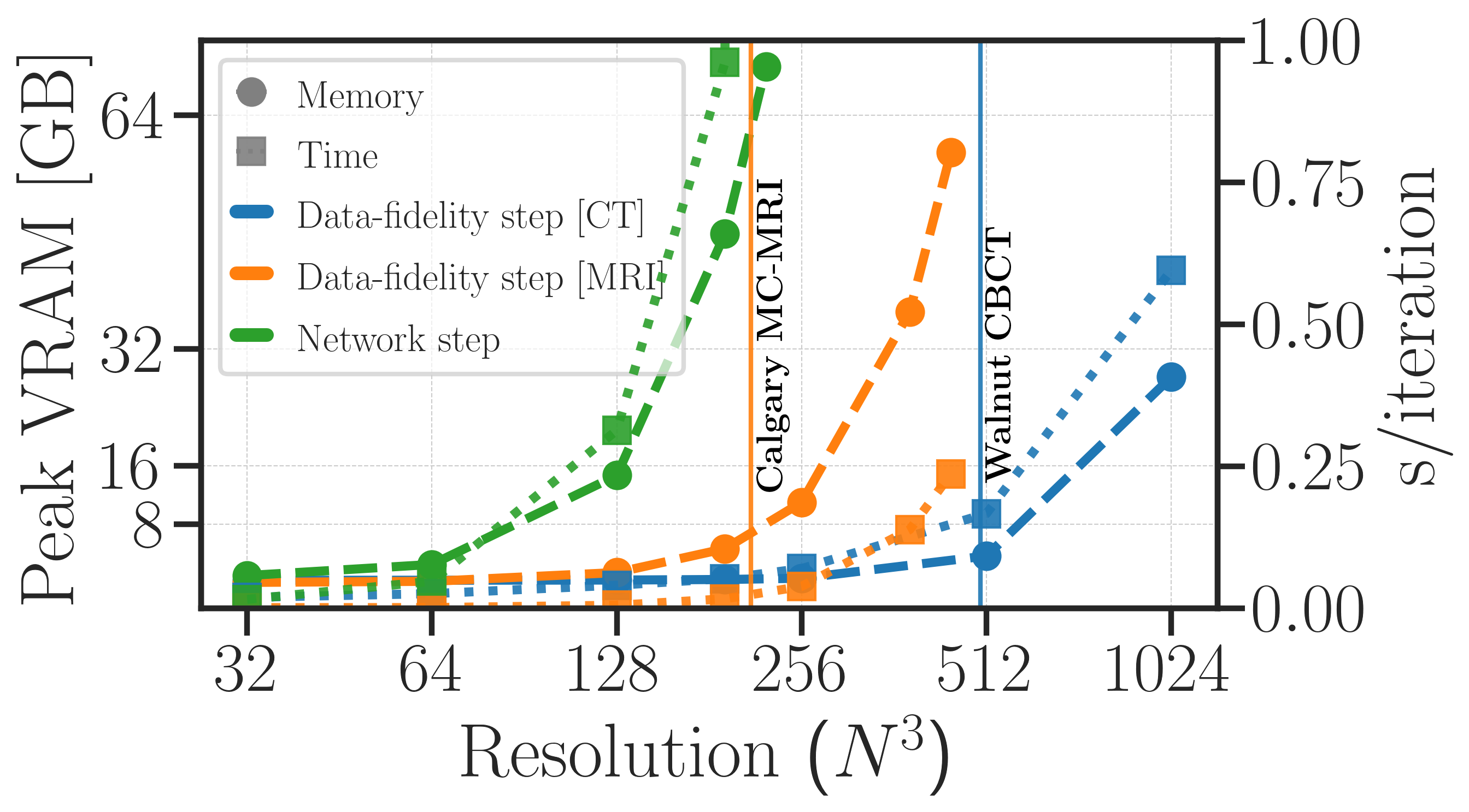
Peak video memory complexity ($\textit{dashed lines}$) and global execution times ($\textit{dotted lines}$) of isolated components used in unrolling. We show the cost of evaluating and back-propagating through a standard 3D data-fidelity step (using gradient descent) and a standard 3D network step (using a 3D DRUNet). We see here that the bottleneck lies in the network step, which grows rapidly with the volume size, while the data-fidelity step remains manageable even at high resolutions.
Method
Domain Partitioning
Let us define the matrices $\mS \in \R^{p \times n}$ and $\mS_\perp \in \R^{q \times n}$ which extracts a vector in $\R^{p}$, respectively in $\R^{q}$, from $ \R^{n}$.
Instead of seeking $\vx^{*}$ entirely, we assume that we know part of the solution, i.e. $\vx_{\text{context}} = \mS_\perp \vx^*$, and we want to recover the remaining part $\vx_{\text{patch}} \in \R^p, ~p \ll n$, such that
\begin{equation}
\vx^{*} = \mS^\top \vx_{\text{patch}} + \mS_{\perp}^\top \vx_{\text{context}},
\end{equation}
By linearity, we can rewrite the global inverse problem in terms of the patch variable $\vx_{\text{patch}}$ as follows
\begin{equation} \label{eq:ip:decomposition}
\begin{aligned}
&\tilde{\vy} = \tilde{\mA} \vx_{\text{patch}}, \\
&\text{where }\tilde{\mA} = \mA \mS^\top \text{ and } \tilde{\vy} = \vy - \mA\mS_{\perp}^\top \vx_{\text{context}}
\end{aligned}
\end{equation}
We have effectively formulated the recovery of a patch of the solution as a smaller inverse problem, which maintains consistency with the global problem. This allows us to train a patch-based network, which significantly reduces the memory complexity of the network step, while keeping the data-fidelity step intact. Akin to patch-based training, we vary the position of the subspace $\rmS \in \R^p$ at random and minimize the following loss
\begin{equation} \label{eq:patch:training}
\begin{aligned}
&\mathcal{L}_{\text{PART}}(\phi) =\E_{\rmS}\E_{\rvx^*, \rvy}~ \| \operatorname{\widetilde{R}}_{\phi}(\tilde{\rvy}, \tilde{\mA}) - \rmS \rvx^{*} \|_2^2, \\
&\text{with } \tilde{\mA} = \mA \mS^\top, \tilde{\vy} = \vy - \mA\mS_{\perp}^\top \mS_{\perp} \vx^{*},
\end{aligned}
\end{equation}
Using our code, training and inference are readily available for any reconstruction pipeline implemented with the DeepInverse library. The partitioning logic can be added in a modular way by wrapping any
deepinv.models.Reconstructor with our proposed PartitionedReconstructor. The partititioned reconstructor takes as input the global measurements $\vy$ and the global operator implemented with physics
import deepinv as dinv

# measurements
y: torch.Tensor

# define the global physics and reconstructor
physics: dinv.physics.LinearPhysics = ...
base_reconstructor: dinv.optim.PGD(...)

patch_size = ...
img_size = ...
stride = tuple(max(1, s // 2) for s in patch_size)  # half-overlap

partitioner = PartitionedReconstructor(
    base_reconstructor=base_reconstructor,
    img_size=img_size,
    patch_size=patch_size,
    stride=stride,
)

x_hat = partitioner(y, physics)
Normal operator approximation with Diagonal-Circulant matrix factorization
With $d$ the squared $\ell_2$-norm, the data-fidelity step of a partitioned problem can written as follows
\begin{align}
\tilde{\vx}_{k+1} &= \tilde{\vx}_{k} - \eta \nabla_{\tilde{\vx}_{k}} d(\tilde{\mA}\tilde{\vx}_{k}, \tilde{\vy}) \notag \\
&=\tilde{\vx}_{k} - \eta \tilde{\mA}^\top (\tilde{\mA}\tilde{\vx}_{k} - \tilde{\vy}), \label{eq:data:step:partitioned} \\
&=\tilde{\vx}_{k} - \eta ( \underbrace{\strut\mS \mA^\top \mA \mS^\top}_{\text{not efficient}} \tilde{\vx}_{k} - \underbrace{\mS \mA^\top \tilde{\vy}}_{\text{pre-computed}}). \notag
\end{align}
In \eqref{eq:data:step:partitioned}, when $\tilde{\vx} \in \R^p$ with $p \ll n$, we would like to avoid using the global normal operator $\mA^\top \mA$.
In this work, we find that a good approximation of the normal operator can be obtained by factorizing it as the product of a diagonal matrix and a circulant matrix, which can be efficiently applied using FFTs. This allows us to significantly reduce the computational cost of the data-fidelity step, while maintaining good reconstruction performance.
\begin{equation} \label{eq:normal:operator:approximation}
\mA^\top \mA \approx \mH = \mathrm{diag}(\vm)^* \mF^{-1} \mathrm{diag}(\bm{\lambda}) \mF \mathrm{diag}(\vm),
\end{equation}
where $\mF$ and $\mF^{-1}$ are the Fourier and inverse Fourier transforms, respectively, $\vm \in \R^{n}$ is homogeneous to spatial sensitivity map, and $\bm{\lambda} \in \mathbb{C}^{n}$ is the frequency response of the convolution kernel associated with $\mA^\top \mA$.
To maintain the computation efficient, we observe that using $\mH$ with a non-symmetric parametrization $\mH = \mathrm{diag}(\vm) \mF^{-1} \mathrm{diag}(\bm{\lambda}) \mF$, works equally well in practice. If needed, the operator $\mH$ can be symmetrized afterwards by computing $\mH_{\text{sym}} = \frac{1}{2}(\mH + \mH^*)$.
The parameters $\vm$ and $\bm{\lambda}$ can be learned end-to-end by minimizing the loss
\begin{align}
\mathcal{L}(\vm, \bm{\lambda}) &= \E_{\rvx \sim \mathcal{N}(\bm{0}, \mI)} \| \mA^\top \mA \rvx - \mH(\vm, \bm{\lambda}) \rvx \|_2^2 \notag\\
&= \| \mA^\top \mA - \mH(\vm, \bm{\lambda}) \|_F^2 \label{eq:frobenius:loss}
\end{align}
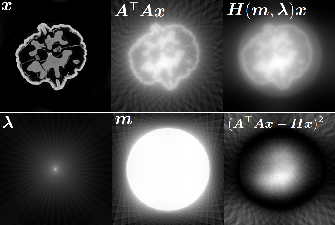
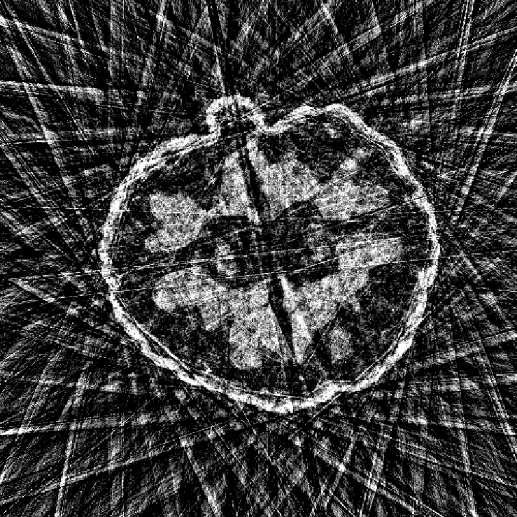
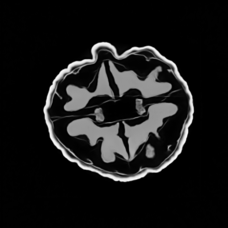
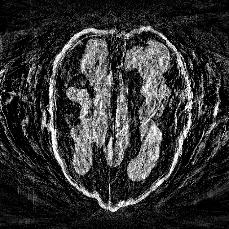
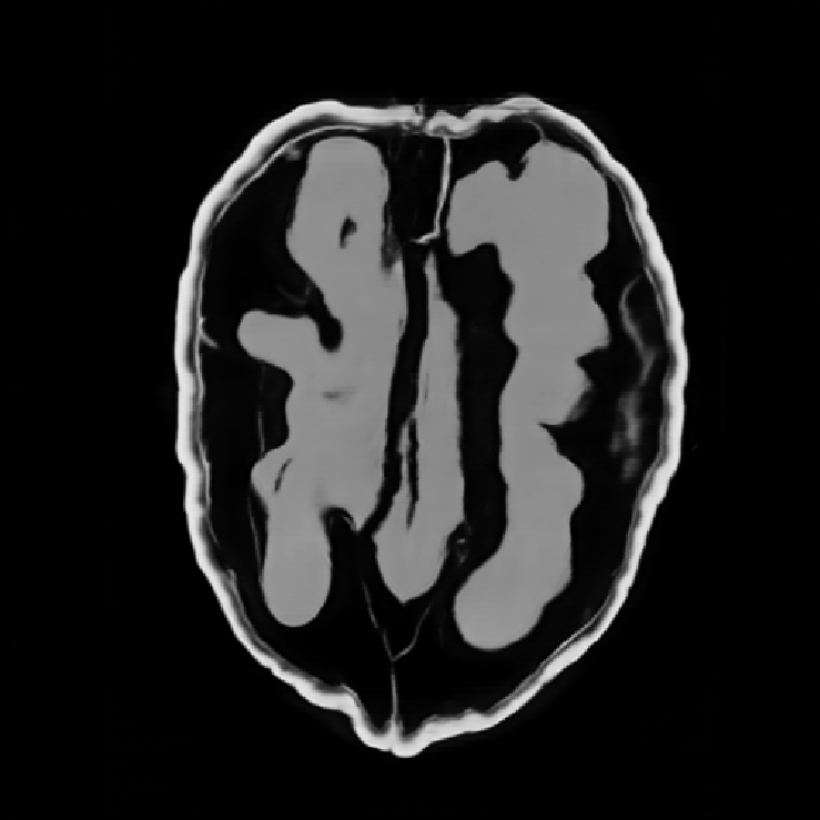
Illustrations of the normal operator approximation on the Walnut-CBCT dataset. (top row) Original volume slice $\vx$, exact normal operator evaluation $\mA^\top \mA \vx$, and approximated normal operator $\mH\vx$. (bottom row) Learned filter $\bm{\lambda}$, learned mask $\vm$, and squared approximation error $(\mA^\top \mA \vx - \mH \vx)^2$.
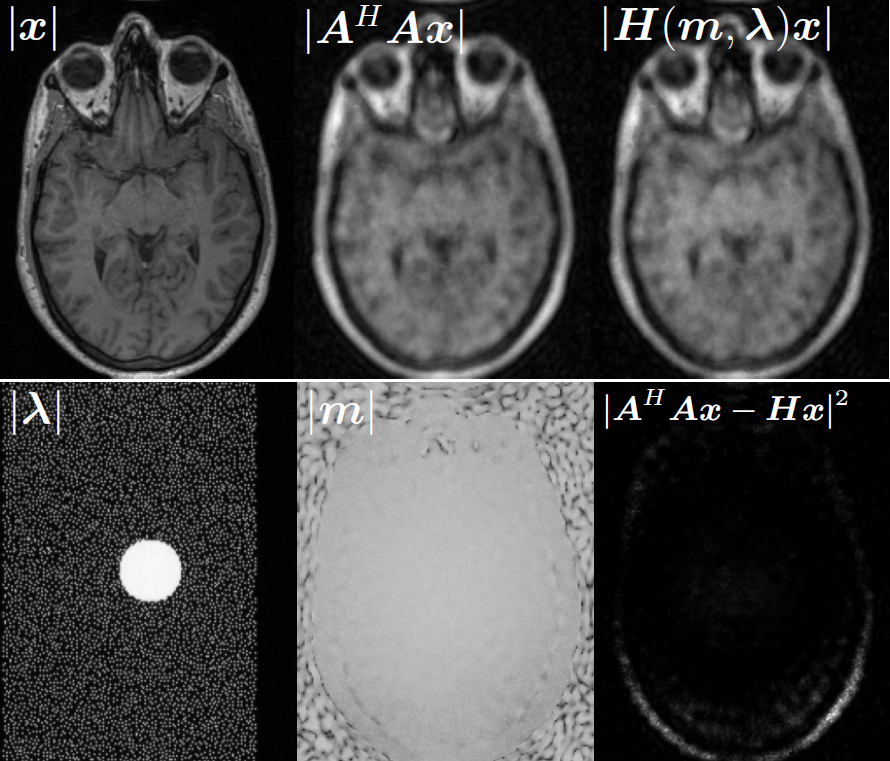
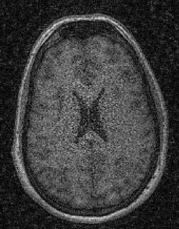
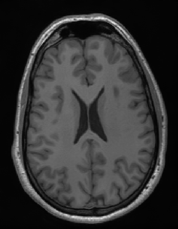
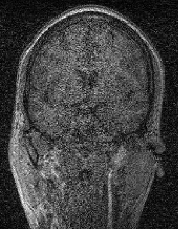
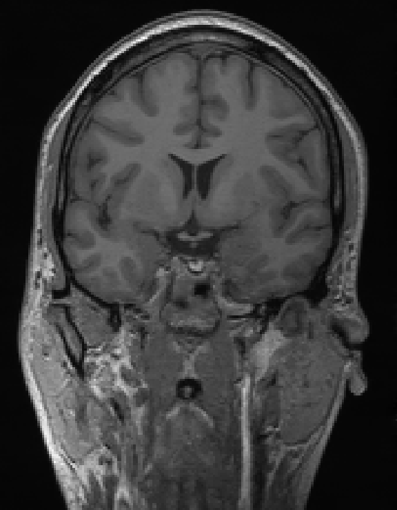
Illustrations of the normal operator approximation on the Calgary-Campinas MCMRI dataset. (top row) Original volume slice $|\vx|$, exact normal operator evaluation $|\mA^H \mA \vx|$, and approximated normal operator $|\mH(\vm, \bm{\lambda}) \vx|$. (bottom row) Learned filter $|\bm{\lambda}|$, learned mask $|\vm|$, and squared approximation error $|\mA^H \mA \vx - \mH \vx|^2$.
Now we can use the approximation $\mH$ instead of the exact normal operator $\mA^\top \mA$ in the partitioned data-fidelity step \eqref{eq:data:step:partitioned}. The factorization $\mH$ admits an efficient evaluation on a small patch by restricting the size of underlying convolution kernel, and by cropping the spatial mask $\vm$ to the patch size.
Similar to the PartitionedReconstructor, we provide a DiagonalCirculantWrapper in our code. It can be used to wrap any deepinv.physics.LinearPhysics operator, and automatically replaces the normal operator with the proposed approximation $\mH$. The wrapper takes as input the global operator implemented with physics, and the parameters $\vm$ and $\bm{\lambda}$ of the approximation, which can be learned end-to-end by minimizing the loss \eqref{eq:frobenius:loss}.
import deepinv as dinv
import torch

# measurements
y: torch.Tensor

# define the global physics and reconstructor
physics: dinv.physics.LinearPhysics = ...
base_reconstructor: dinv.optim.PGD(...)

# define the partitioner
partitioner = PartitionedReconstructor(...)

# assuming the approximation parameters are already learned, we can wrap the physics as follows
spatial_mask: torch.Tensor
fourier_filter: torch.Tensor

wrapped_physics = DiagCirculantWrapper(
    physics=physics,
    img_size=physics.img_size,
    scaling=1., # scale with the spectral norm |A|² if the operator is not normalized
    device=device,
)

x_hat = partitioner(
    y,
    wrapped_physics,
    fourier_filter=fourier_filter,
    spatial_mask=spatial_mask,
)
Results
Qualitative results
Quantitative Results
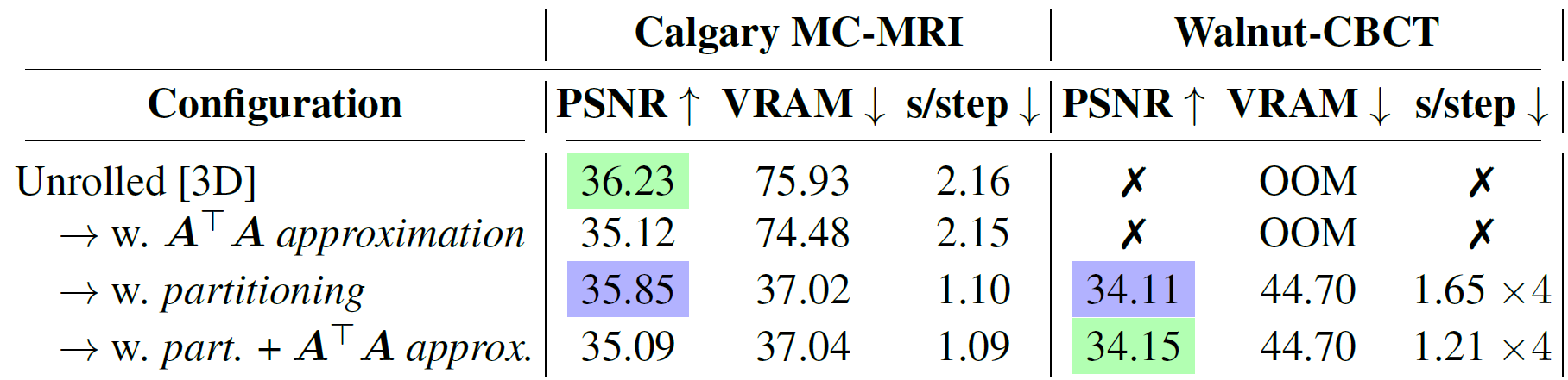
Ablation study. For each line we report the PSNR averaged on the different subsampling configurations, as well as the peak video memory usage in GB and training speed. Best and second-best results highlighted.
Citation
@article{vo2026efficient,
            title={Efficient Unrolled Networks for Large-Scale 3D Inverse Problems},
            author={Romain Vo and Julián Tachella},
            journal={arXiv preprint arXiv:2601.02141},
            year={2026}
        }